
The test comparing two independent population means with unknown and possibly unequal population standard deviations is called the Aspin-Welch \(t\)-test. The degrees of freedom formula was developed by Aspin-Welch.
The comparison of two population means is very common. A difference between the two samples depends on both the means and the standard deviations. Very different means can occur by chance if there is great variation among the individual samples. In order to account for the variation, we take the difference of the sample means, \(\bar_ - \bar_\), and divide by the standard error in order to standardize the difference. The result is a t-score test statistic.
Because we do not know the population standard deviations, we estimate them using the two sample standard deviations from our independent samples. For the hypothesis test, we calculate the estimated standard deviation, or standard error, of the difference in sample means, \(\bar_ - \bar_\).
The standard error is:
The test statistic (t-score) is calculated as follows:
The number of degrees of freedom (\(df\)) requires a somewhat complicated calculation. However, a computer or calculator calculates it easily. The \(df\) are not always a whole number. The test statistic calculated previously is approximated by the Student's t-distribution with \(df\) as follows:
We can also use a conservative estimation of degree of freedom by taking DF to be the smallest of \(n_-1\) and \(n_-1\)
When both sample sizes \(n_\) and \(n_\) are five or larger, the Student's t approximation is very good. Notice that the sample variances \((s_)^\) and \((s_)^\) are not pooled. (If the question comes up, do not pool the variances.)
It is not necessary to compute the degrees of freedom by hand. A calculator or computer easily computes it.
The average amount of time boys and girls aged seven to 11 spend playing sports each day is believed to be the same. A study is done and data are collected, resulting in the data in Table \(\PageIndex\). Each populations has a normal distribution.
| Sample Size | Average Number of Hours Playing Sports Per Day | Sample Standard Deviation | |
|---|---|---|---|
| Girls | 9 | 2 | 0.8660.866 |
| Boys | 16 | 3.2 | 1.00 |
Is there a difference in the mean amount of time boys and girls aged seven to 11 play sports each day? Test at the 5% level of significance.
Answer
The population standard deviations are not known. Let g be the subscript for girls and b be the subscript for boys. Then, \(\mu_\) is the population mean for girls and \(\mu_\) is the population mean for boys. This is a test of two independent groups, two population means.
Random variable: \(\bar_ - \bar_ =\) difference in the sample mean amount of time girls and boys play sports each day.
The words "the same" tell you \(H_\) has an "=". Since there are no other words to indicate \(H_\), assume it says "is different." This is a two-tailed test.
Distribution for the test: Use \(t_\) where \(df\) is calculated using the \(df\) formula for independent groups, two population means. Using a calculator, \(df\) is approximately 18.8462. Do not pool the variances.
Calculate the p-value using a Student's t-distribution: \(p\text = 0.0054\)
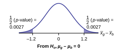
Graph:
 right of x = 1.2 are shaded to represent the p-value. The area of each region is 0.0028." width="488px" height="208px" />
\[\bar_ - \bar_ = 2 - 3.2 = -1.2\]
Half the \(p\text\) is below –1.2 and half is above 1.2.
Make a decision: Since \(\alpha > p\text\), reject \(H_\). This means you reject \(\mu_ = \mu_\). The means are different.
Press STAT . Arrow over to TESTS and press 4:2-SampTTest . Arrow over to Stats and press ENTER . Arrow down and enter 2 for the first sample mean, \(\sqrt\) for Sx1, 9 for n1, 3.2 for the second sample mean, 1 for Sx2, and 16 for n2. Arrow down to μ1: and arrow to does not equal μ2. Press ENTER . Arrow down to Pooled: and No . Press ENTER . Arrow down to Calculate and press ENTER . The \(p\text\) is \(p = 0.0054\), the dfs are approximately 18.8462, and the test statistic is -3.14. Do the procedure again but instead of Calculate do Draw.
Conclusion: At the 5% level of significance, the sample data show there is sufficient evidence to conclude that the mean number of hours that girls and boys aged seven to 11 play sports per day is different (mean number of hours boys aged seven to 11 play sports per day is greater than the mean number of hours played by girls OR the mean number of hours girls aged seven to 11 play sports per day is greater than the mean number of hours played by boys).
Two samples are shown in Table. Both have normal distributions. The means for the two populations are thought to be the same. Is there a difference in the means? Test at the 5% level of significance.
| Sample Size | Sample Mean | Sample Standard Deviation | |
|---|---|---|---|
| Population A | 25 | 5 | 1 |
| Population B | 16 | 4.7 | 1.2 |
Answer
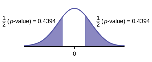
The \(p\text\) is \(0.4125\), which is much higher than 0.05, so we decline to reject the null hypothesis. There is not sufficient evidence to conclude that the means of the two populations are not the same.
When the sum of the sample sizes is larger than \(30 (n_ + n_ > 30)\) you can use the normal distribution to approximate the Student's \(t\).
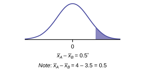
A study is done by a community group in two neighboring colleges to determine which one graduates students with more math classes. College A samples 11 graduates. Their average is four math classes with a standard deviation of 1.5 math classes. College B samples nine graduates. Their average is 3.5 math classes with a standard deviation of one math class. The community group believes that a student who graduates from college A has taken more math classes, on the average. Both populations have a normal distribution. Test at a 1% significance level. Answer the following questions.
Solutions

A study is done to determine if Company A retains its workers longer than Company B. Company A samples 15 workers, and their average time with the company is five years with a standard deviation of 1.2. Company B samples 20 workers, and their average time with the company is 4.5 years with a standard deviation of 0.8. The populations are normally distributed.
Answer
A professor at a large community college wanted to determine whether there is a difference in the means of final exam scores between students who took his statistics course online and the students who took his face-to-face statistics class. He believed that the mean of the final exam scores for the online class would be lower than that of the face-to-face class. Was the professor correct? The randomly selected 30 final exam scores from each group are listed in Table \(\PageIndex\) and Table \(\PageIndex\).
| 67.6 | 41.2 | 85.3 | 55.9 | 82.4 | 91.2 | 73.5 | 94.1 | 64.7 | 64.7 |
| 70.6 | 38.2 | 61.8 | 88.2 | 70.6 | 58.8 | 91.2 | 73.5 | 82.4 | 35.5 |
| 94.1 | 88.2 | 64.7 | 55.9 | 88.2 | 97.1 | 85.3 | 61.8 | 79.4 | 79.4 |
| 77.9 | 95.3 | 81.2 | 74.1 | 98.8 | 88.2 | 85.9 | 92.9 | 87.1 | 88.2 |
| 69.4 | 57.6 | 69.4 | 67.1 | 97.6 | 85.9 | 88.2 | 91.8 | 78.8 | 71.8 |
| 98.8 | 61.2 | 92.9 | 90.6 | 97.6 | 100 | 95.3 | 83.5 | 92.9 | 89.4 |
Is the mean of the Final Exam scores of the online class lower than the mean of the Final Exam scores of the face-to-face class? Test at a 5% significance level. Answer the following questions:
(See the conclusion in Example, and write yours in a similar fashion)
Be careful not to mix up the information for Group 1 and Group 2!
Answer

First put the data for each group into two lists (such as L1 and L2). Press STAT. Arrow over to TESTS and press 4:2SampTTest. Make sure Data is highlighted and press ENTER. Arrow down and enter L1 for the first list and L2 for the second list. Arrow down to \(\mu_\): and arrow to \(\neq \mu_\) (does not equal). Press ENTER. Arrow down to Pooled: No. Press ENTER. Arrow down to Calculate and press ENTER.
Cohen's \(d\) is a measure of effect size based on the differences between two means. Cohen’s \(d\), named for United States statistician Jacob Cohen, measures the relative strength of the differences between the means of two populations based on sample data. The calculated value of effect size is then compared to Cohen’s standards of small, medium, and large effect sizes.
| Size of effect | \(d\) |
|---|---|
| Small | 0.2 |
| medium | 0.5 |
| Large | 0.8 |
Cohen's \(d\) is the measure of the difference between two means divided by the pooled standard deviation: \(d = \dfrac_-\bar_>>>\) where \(s_ = \sqrt<\dfrac<(n_-1)s^_ + (n_-1)s^_>
Calculate Cohen’s d for Example. Is the size of the effect small, medium, or large? Explain what the size of the effect means for this problem.
Answer
\(\mu_ = 4 s_ = 1.5 n_ = 11\)
\(\mu_ = 3.5 s_ = 1 n_ = 9\)
The effect is small because 0.384 is between Cohen’s value of 0.2 for small effect size and 0.5 for medium effect size. The size of the differences of the means for the two colleges is small indicating that there is not a significant difference between them.
Calculate Cohen’s \(d\) for Example. Is the size of the effect small, medium or large? Explain what the size of the effect means for this problem.
Answer
\(d = 0.834\); Large, because 0.834 is greater than Cohen’s 0.8 for a large effect size. The size of the differences between the means of the Final Exam scores of online students and students in a face-to-face class is large indicating a significant difference.
Weighted alpha is a measure of risk-adjusted performance of stocks over a period of a year. A high positive weighted alpha signifies a stock whose price has risen while a small positive weighted alpha indicates an unchanged stock price during the time period. Weighted alpha is used to identify companies with strong upward or downward trends. The weighted alpha for the top 30 stocks of banks in the northeast and in the west as identified by Nasdaq on May 24, 2013 are listed in Table and Table, respectively.
| 94.2 | 75.2 | 69.6 | 52.0 | 48.0 | 41.9 | 36.4 | 33.4 | 31.5 | 27.6 |
| 77.3 | 71.9 | 67.5 | 50.6 | 46.2 | 38.4 | 35.2 | 33.0 | 28.7 | 26.5 |
| 76.3 | 71.7 | 56.3 | 48.7 | 43.2 | 37.6 | 33.7 | 31.8 | 28.5 | 26.0 |
| 126.0 | 70.6 | 65.2 | 51.4 | 45.5 | 37.0 | 33.0 | 29.6 | 23.7 | 22.6 |
| 116.1 | 70.6 | 58.2 | 51.2 | 43.2 | 36.0 | 31.4 | 28.7 | 23.5 | 21.6 |
| 78.2 | 68.2 | 55.6 | 50.3 | 39.0 | 34.1 | 31.0 | 25.3 | 23.4 | 21.5 |
Is there a difference in the weighted alpha of the top 30 stocks of banks in the northeast and in the west? Test at a 5% significance level. Answer the following questions:
Answer

Two population means from independent samples where the population standard deviations are not known
Degrees of freedom:
OR use the DF to be the smallest of \(n_-1\) and \(n_-1\)
Cohen’s \(d\) is the measure of effect size:
This page titled 9.2: Comparing Two Independent Population Means (Hypothesis test) is shared under a CC BY 4.0 license and was authored, remixed, and/or curated by Zoya Kravets via source content that was edited to the style and standards of the LibreTexts platform.